Introduction

Think of machine learning as teaching your computer a magic trick. It's a type of artificial intelligence (AI) that allows software applications to become more accurate in predicting outcomes without being explicitly programmed to do so.

Machine learning is broadly categorized into supervised and unsupervised, with the former referring to predicting the unknown using what is currently known. In other words, supervised learning relies upon “right answers,” which are used to train a model from which it learns and can subsequently be used in predicting outcomes from input data. On the other hand, unsupervised learning allows the model to work independently to discover information; it's not given the "right answer.”

Machine learning is about creating algorithms and systems that can improve their own performance through learning and experience. It's a rapidly evolving field and plays a key role in many aspects of modern life, from recommending the next movie you should watch, to predicting stock market trends, to even helping doctors diagnose diseases. It's a pretty exciting space, I must say!

Now let’s dive in and understand what is classification in machine learning.

Definition and Explanation of Classification in Machine Learning

To start with, you must be wondering what classification implies and especially where it comes in within the context of machine learning. First, imagine you're sorting laundry into different categories - shirts, pants, socks, and so on. You're basically classifying your laundry items, right? It's a similar concept in machine learning, albeit a bit more complex.
In machine learning, classification is a supervised learning approach, which you might remember as the one where we provide the machine with the "right answers" to learn from. What we're doing here is training our model to predict or categorize class labels, which are the "categories," for new, unseen data, based on what it has learned from the training data.

For instance, you could have a bunch of emails, and you want to classify them as either "spam" or "not spam." You train your model on a dataset where you already know which emails are spam and which aren't. The model then learns this dataset's characteristics of spam and non-spam emails. Once trained, you can give it a new set of emails it's never seen before, and it should be able to classify them into "spam" or "not spam" based on what it has learned.

There are various algorithms used for classification tasks. Some popular ones are logistic regression, decision trees, support vector machines, and k-nearest neighbors. Each has its way of learning from data and making the final decision.

Importance and Applications of Classification in various industries

First, classification plays a vital role across numerous sectors because it helps us make sense of vast amounts of data. We can identify patterns and trends that help drive strategic decisions by categorizing this data. Now, onto some specific applications:

• Healthcare: Classification is a game-changer here. It's used to predict whether a patient has a particular disease based on their symptoms. For example, machine learning models can be trained to classify tumors as benign or malignant based on medical imaging. This helps in early detection and effective treatment.

• Finance: Banks and financial institutions use classification to predict whether a customer will default on a loan. This helps them manage risk and make informed lending decisions. It's also used in fraud detection, classifying transactions as legitimate or fraudulent.

• Marketing: Ever wondered how you get those eerily accurate product recommendations? Classification algorithms are at work, grouping customers based on their behavior and preferences to provide personalized recommendations and enhance customer experience. It can be used in marketing analytics to classify customers into two categories: 'will churn' and 'will not churn.' The 'will churn' category represents customers likely to discontinue a service soon, while the 'will not churn' category represents customers likely to continue with the service.

• Transportation: Machine learning classification helps predict whether a flight will be delayed based on factors such as weather conditions, previous flight data, and so on. This helps airlines manage their schedules more effectively and keeps passengers informed.

• Cybersecurity: Here, classification is used to identify and categorize harmful cyber threats according to their threat level. This helps in faster response and prevention of potential breaches.

• Social Media: Platforms like Twitter or Facebook use classification to filter out inappropriate content or identify and remove hate speech or bullying. They also use it to categorize your interests and show you relevant ads.

Types of Classification Algorithms

Classification algorithms are basically the means through which classification can be carried out. In other words, it defines an approach used to predict the category, or class, of an item or sample based on certain features. The following are the types of algorithms:

• Logistic Regression

• Decision Trees

• Random Forests

• Support Vector Machines

• K-Nearest Neighbors

• Naive Bayes

Let’s describe them further:

Logistic Regression: Despite its name, it is used for classification, not regression tasks. It uses a logistic function to model the probability of a particular class or event. For example, it can predict whether an email is spam (1) or not spam (0) based on features like the presence of certain words.

Decision Trees: This algorithm is a bit like playing the game of "20 Questions". It makes decisions by asking a series of questions, each narrowing down the possibilities until a final decision is made. For example, a decision tree could classify whether an animal is a dog or not by asking questions like "Does it have fur?" or "Does it bark?".

Random Forests: As the name suggests, this algorithm is a 'forest' of decision trees. It creates a bunch of different decision trees on randomly selected data samples, gets predictions from each tree, and selects the best solution through voting. It's a great way to avoid overfitting, which happens when a model learns the training data too well and performs poorly on unseen data.

Support Vector Machines (SVM): SVM is a bit more complex. It classifies data by finding the best hyperplane that separates all data points of one class from those of the other class. The best hyperplane is the one that represents the largest separation or margin between the two classes. Think of it like drawing a line in the sand between two groups of data points.

K-Nearest Neighbors (KNN): This algorithm is all about proximity. It classifies a data point based on how its neighbors are classified. KNN stores all available cases and classifies new cases by a majority vote of its k neighbors. The case being assigned to the class is most common among its K nearest neighbors measured by a distance function.

Naive Bayes: Named after Bayes' theorem, this algorithm simplifies the process of predicting a class label by assuming that the features are independent of each other. Despite its simplicity and the 'naive' assumption of independence, Naive Bayes can be particularly effective in text classification, like deciding whether an email is spam or not.

Implementing K-Nearest Neighbors with Python

Now let's dive into how to implement the K-Nearest Neighbors (KNN) algorithm using Python. For this guide, we'll use the popular machine learning library scikit-learn. In this example, I used the iris dataset, popularly used in EDA, and data science examples.

Tools and Libraries Required

First, we need to import the necessary Python libraries for our task. These include:

import numpy as np import pandas as pd import matplotlib.pyplot as plt import seaborn as sns from sklearn.model_selection import train_test_split from sklearn.preprocessing import StandardScaler from sklearn.neighbors import KNeighborsClassifier from sklearn.metrics import confusion_matrix, accuracy_score from sklearn.model_selection import GridSearchCV from sklearn.model_selection import cross_val_score from sklearn.metrics import classification_report

numpy and pandas are fundamental packages for scientific computing and data manipulation in Python. matplotlib and seaborn are used for data visualization. sklearn (or scikit-learn) is a library in Python that provides many unsupervised and supervised learning algorithms.

Loading and Exploring the Dataset

We load the Iris dataset into a DataFrame, which allows us to manipulate the data easily:

# Load the Iris dataset df = pd.read_csv('./iris.csv') # Display the first 5 rows of the dataset df.head()

This returns:

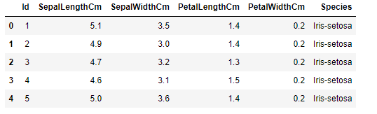
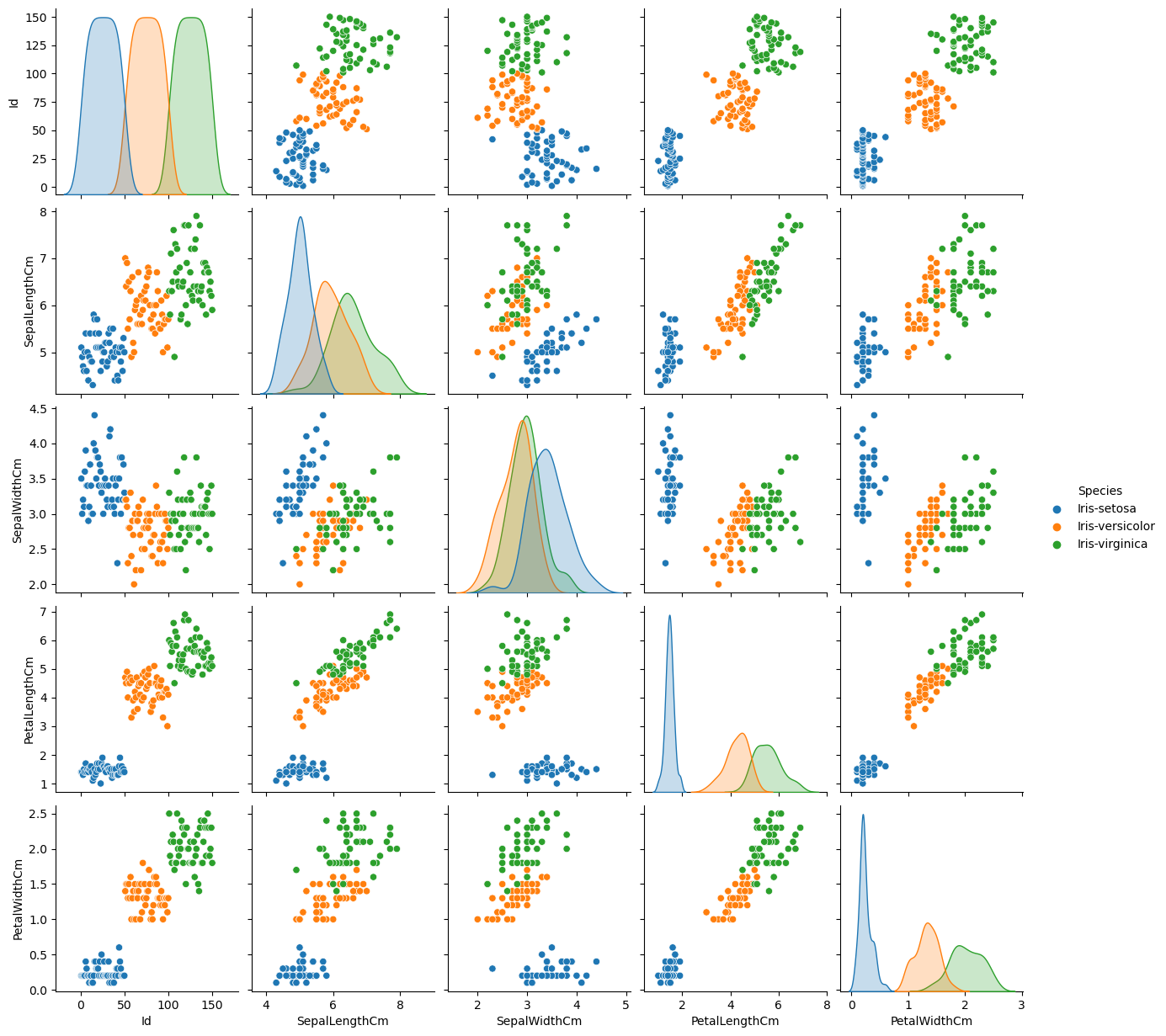
Our dataset consists of 150 samples from each of three species of Iris flowers (Iris setosa, Iris virginica, and Iris versicolor). Four features were measured from each sample: the lengths and the widths of the sepals and petals.

Next, we check for missing values:

# Check for missing values in each column df.isnull().sum()

Fortunately, our dataset contains no missing values, so there is no need for any data-cleaning steps.

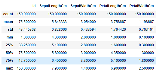
Let's get some statistical details of the dataset:

df.describe()

We can also check the balance of our dataset by looking at the distribution of species:

#show value counts by species df['Species'].value_counts()

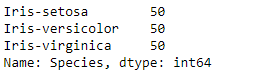
The result shows that our dataset is perfectly balanced with 50 instances for each species.

Visualizing the Data

To understand our data better, let's visualize the pairplot of different features in our DataFrame. This allows us to see the distribution of single variables and relationships between two variables.

sns.pairplot(df, hue='Species')

This will provide us with a set of scatter plots which can be helpful to understand the data distribution and correlation of different variables in the dataset.

Preparing the Data

Before feeding the data into the model, we have to split it into features (X) and target (y) variables:

#assignment of features and labels (targets) to variables: X = df.iloc[:, 1:5].values #features y = df.iloc[:, 5].values  #target

The features are the independent variables. Here, they are the physical measurements of the flowers. On the other hand, the target is the dependent variable, the species of the flowers.

Our target variable is categorical. To convert this categorical data into a model-understandable numerical format, we use LabelEncoder from sklearn.preprocessing:

from sklearn.preprocessing import LabelEncoder le = LabelEncoder() y = le.fit_transform(y)

The rest of the steps and code associated with them will be discussed in the next parts of the article. This includes data splitting, feature scaling, model definition and training, prediction, model evaluation, and optimization with grid search.

Splitting the Dataset

The next step is to split our data into training and testing datasets. The training set is used to train the model, while the test set is used to evaluate the performance of the model. We do this using the train_test_split function from sklearn.model_selection. We use 70% of the data for training and 30% for testing:

# Split the dataset into training set and test set X_train, X_test, y_train, y_test = train_test_split(X, y, test_size = 0.3, random_state = 0)

Feature Scaling

Before making any actual predictions, it is always a good practice to scale the features so that all of them can be uniformly evaluated. Feature scaling is performed only on the training data and not on the test data. This is because in the real world, data (test set) is not scaled and the ultimate purpose of the neural network is to make predictions on real-world data. We use StandardScaler from sklearn.preprocessing:

# Perform feature scaling scaler = StandardScaler() X_train = scaler.fit_transform(X_train) X_test = scaler.transform(X_test)

Building the KNN Model

Next, we define the KNN model and the parameters to search. For KNN, the most important parameter is the number of neighbors, n_neighbors. We will use GridSearchCV from sklearn.model_selection to find the optimal number of neighbors:

# Define the model and parameters to search knn = KNeighborsClassifier() parameters = {'n_neighbors': np.arange(1, 10)}

Training the Model and Hyperparameter Tuning

We now train our model and perform hyperparameter tuning using grid search:

# Use GridSearchCV grid = GridSearchCV(knn, parameters, cv=10) grid.fit(X_train, y_train)

Once the model is trained, we can get the best parameters:

# Get the best parameters best_params = grid.bestparams best_knn_model = grid.bestestimator

Making Predictions

Now that our model is trained, we can use it to make predictions:

# Make predictions y_pred = best_knn_model.predict(X_test)

And we can use the model to predict the species of a new iris sample:

# Assuming your features are in the order: sepal length, sepal width, petal length, petal width new_iris = np.array([[3, 5, 4, 2]]) # Use the model to make a prediction new_iris_pred = best_knn_model.predict(new_iris) # To make it human-readable, map the encoded prediction back to the original label new_iris_species = le.inverse_transform(new_iris_pred) print(f"The iris is predicted to be of the species: {new_iris_species[0]}")

This returns: The iris is predicted to be of the species: Iris-virginica

Evaluating the Model

We can evaluate our model by calculating the accuracy and generating a confusion matrix:

# Evaluate the model accuracy = accuracy_score(y_test, y_pred) conf_matrix = confusion_matrix(y_test, y_pred) print(f"Model Accuracy: {accuracy}") print(f"Confusion Matrix: \n{conf_matrix}")

This returns:

Model Accuracy: 0.9777777777777777 Confusion Matrix: [[16  0  0] [ 0 17  1] [ 0  0 11]]

This suggests that the model accuracy is 97% which is good.

We can also use cross-validation to get a better measure of model's accuracy:

# Cross-validation cv_scores = cross_val_score(best_knn_model, X, y, cv=10) print(f"CV average score: {cv_scores.mean()}")

Finally, we can generate a classification report, which provides important metrics such as precision, recall, and f1-score:

# Classification Report print(classification_report(y_test, y_pred, target_names=df['Species'].unique()))

In the classification report, "precision" is the ability of the classifier not to label as positive a sample that is negative, "recall" is the ability of the classifier to find all the positive samples, and the F-beta score is the harmonic average of precision and recall. The "support" is the number of occurrences of each class in y_test.

Conclusion

Through the K-Nearest Neighbors classification algorithm, we are able to create a model that can predict the species of iris with high accuracy. It shows how effective machine learning can be for tasks like this.

Thank you for taking the time to read through this comprehensive guide on implementing the K-Nearest Neighbors classification algorithm using Python. We've covered a lot of ground, from understanding the Iris dataset, data preprocessing, to training the model, and finally evaluating its performance.

I appreciate your time and interest in this subject matter, and I look forward to hearing your thoughts and feedback. If you have any questions or comments about the steps we've gone through or the code used, please don't hesitate to share. I'm always keen to learn from your insights and experiences, and your feedback will help make this guide better for everyone.

Explore the notebook: https://github.com/kaydata/Classification-using-K-K-Nearest-Neighbors-KNN-